(This is a draft and truncated version - for final and full version, see
Concise Encyclopedia of Biostatistics for Medical Professionals)
quantiles, see also percentiles and percentile curves
Quantiles are the values of the variable that divide the total number of subjects into ordered groups of equal size. These are also called fractiles. This means that each group so formed will have same number of subjects. In general, the values dividing subjects into S equal groups may be called the S-tiles. The total number of S-tiles is (S – 1) as the last S-tile is the maximum value itself. For example, median is the value such that the number of subjects with value more than the median is the same as the number of subjects less than the median –this is a quantile that divides the subjects into two equal groups. Tertiles divide the subjects into three equal groups, quartiles into four equal groups, quintiles into five equal groups, deciles into ten equal groups, vigintiles into 20 equal groups, and percentiles into 100 equal groups. For example, 9th decile is the minimum value below which at least 90% of the values lay and not more than 10% values will be greater.
Evidently quantiles are primarily meant to be used with quantitative, particularly continuous data. A value xp is the pth S-tile if P(x ≤ xp) = p/S. For example, for a standard Gaussian (Normal) distribution, 97.5th percentile is 1.96 since P(z ≤ 1.96) = 0.975, and second tertile is that value of a for which P(z ≤ a) = 2/3. Normal distribution gives a = 0.43. Note the equality sign. If the values are quantitative but discrete such as parity, months of gestation, and ranks, quantiles may not be fully defined. This can happen with continuous values also in samples, especially when the sample size is small. Quantiles in ungrouped data are obtained simply in the following manner:
pth S-tile = (p*n/S)the value in ascending order of magnitude,
where n is the total number of subjects. For n = 200 subjects,
35th percentile = (35×200/100) = 70th value,
7th decile = (7×200/10) = 140th value,
3rd quintile = (3×200/5) = 120th value,
1st quartile = (1×200/4) = 50th value, and
2nd tertile = (2×200/3) = 133rd value,
in ascending order of magnitude.
Percentiles can be denoted by P1, P2, P3, etc., deciles by D1, D2, D3, etc., and quartiles by Q1, Q2, and Q3. A feature worth noting for all quantiles is that quantile of (x + y) ≠ quantile of x + quantile of y. This needs to be understood in the context of mean since mean(x + y) = mean(x) + mean(y).
Consider the following 18 values:
23, 12, 56, 25, 34, 43, 12, 7, 49, 27, 34, 45, 28, 14, 19, 17, 16, 28.
After ordering, these are: 7, 12, 12, 14, 16, 17, 19, 23, 25, 27, 28, 28, 34, 34, 43, 45, 49, 56. Thus 3rd quartile is the 18×3/4 = 13.5th value. Since the 13th value is 34 and the 14th value is also 34, the 3rd quartile is (34+34)/2 = 34. Similarly 4th quintile is the 18×4/5 = 14.4th value and obtained as 4/10th away from the 14th value. Since the 14th value is 34 and the 15th value is 43, 4/10th apportion of the difference of 9 between these two values is 3.6, giving 4th quintile = 34 + 3.6 = 37.6. In most practical applications, decimals are approximated, i.e., 14th value is taken as 14.4th value.
Quantiles in Grouped Data
In case of grouped data, the calculation is based mainly on the quantile interval—the interval containing the required quantile.
Grouped data:
where ap–1 is the lower limit of the quantile interval. The quantile interval is the one containing the (p*n/S)th observation in order of magnitude,
C = cumulative frequency until the quantile interval,
fp = frequency in the quantile interval, and
hp = width of the quantile interval.
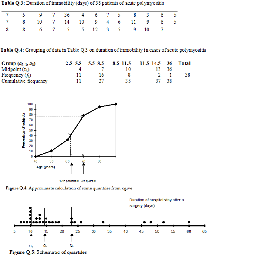
Consider the duration of immobility data in Table Q.3. The 2nd tertile in this data set is approximately 2×38/3 = 25th value in ascending order. This is 8 days. Also, 85th percentile = (85×38/100)th or 32nd value in ascending order = 10 days. The same data are grouped in Table Q.4. The 25th value is in the interval (5.5–8.5) days. Thus, for the 2nd tertile, ap–1 = 5.5, C = 11, fp = 16, and hp = 3. Therefore,
2nd tertile (grouped data) = 5.5 + 3*(25 - 11)/16 = 8.1 days.
Similarly, 85th percentile (grouped data) = 8.5 + 3*(32 - 27)/8 = 10.4 days.
The other method for obtaining approximate quantiles in case of grouped data is graphical. For graphical calculation of quantiles, the cumulative percentages of subjects are plotted against the upper end of the data intervals, called the ogive. Suppose for an age distribution, this plot is as shown in Figure Q.4. The cumulative percentages for age –49, –59, –69, –79, and beyond 79 are 11, 32, 78, 95, and 100, respectively. To obtain a pth S-tile, draw a horizontal line at 100p/S% and read the value on the x-axis where this horizontal line intersects the percent-based ogive. Figure Q.4 shows the 40th percentile and the 3rd quartile of age for these data. The calculations in the case of grouped data are, in any case, approximate for quantiles just as for the mean, median, and mode – thus graphic method may not be as bad for quantiles too.
Interpretation of the Quantiles
All calculations can be done with the help of computers, but the method of computation helps in understanding quantiles and their proper interpretation. Figure Q.5 on quartiles may provide another perspective. This shows the duration of hospital stay after surgery for 30 patients. See how quartiles are determined. They divide the total number of subjects into four equal groups in terms of frequency. These frequencies may not be exactly equal in the case of the discrete data depicted in Figure Q.5 but would be equal in the case of really continuous data. Other quantiles have similar interpretations.
Quantiles are sometimes used for an objective categorization of the subjects. ... ...
For final and full version, see
Concise Encyclopedia of Biostatistics for Medical Professionals
Concise Encyclopedia of Biostatistics for Medical Professionals)
quantiles, see also percentiles and percentile curves
Quantiles are the values of the variable that divide the total number of subjects into ordered groups of equal size. These are also called fractiles. This means that each group so formed will have same number of subjects. In general, the values dividing subjects into S equal groups may be called the S-tiles. The total number of S-tiles is (S – 1) as the last S-tile is the maximum value itself. For example, median is the value such that the number of subjects with value more than the median is the same as the number of subjects less than the median –this is a quantile that divides the subjects into two equal groups. Tertiles divide the subjects into three equal groups, quartiles into four equal groups, quintiles into five equal groups, deciles into ten equal groups, vigintiles into 20 equal groups, and percentiles into 100 equal groups. For example, 9th decile is the minimum value below which at least 90% of the values lay and not more than 10% values will be greater.
Evidently quantiles are primarily meant to be used with quantitative, particularly continuous data. A value xp is the pth S-tile if P(x ≤ xp) = p/S. For example, for a standard Gaussian (Normal) distribution, 97.5th percentile is 1.96 since P(z ≤ 1.96) = 0.975, and second tertile is that value of a for which P(z ≤ a) = 2/3. Normal distribution gives a = 0.43. Note the equality sign. If the values are quantitative but discrete such as parity, months of gestation, and ranks, quantiles may not be fully defined. This can happen with continuous values also in samples, especially when the sample size is small. Quantiles in ungrouped data are obtained simply in the following manner:
pth S-tile = (p*n/S)the value in ascending order of magnitude,
where n is the total number of subjects. For n = 200 subjects,
35th percentile = (35×200/100) = 70th value,
7th decile = (7×200/10) = 140th value,
3rd quintile = (3×200/5) = 120th value,
1st quartile = (1×200/4) = 50th value, and
2nd tertile = (2×200/3) = 133rd value,
in ascending order of magnitude.
Percentiles can be denoted by P1, P2, P3, etc., deciles by D1, D2, D3, etc., and quartiles by Q1, Q2, and Q3. A feature worth noting for all quantiles is that quantile of (x + y) ≠ quantile of x + quantile of y. This needs to be understood in the context of mean since mean(x + y) = mean(x) + mean(y).
Consider the following 18 values:
23, 12, 56, 25, 34, 43, 12, 7, 49, 27, 34, 45, 28, 14, 19, 17, 16, 28.
After ordering, these are: 7, 12, 12, 14, 16, 17, 19, 23, 25, 27, 28, 28, 34, 34, 43, 45, 49, 56. Thus 3rd quartile is the 18×3/4 = 13.5th value. Since the 13th value is 34 and the 14th value is also 34, the 3rd quartile is (34+34)/2 = 34. Similarly 4th quintile is the 18×4/5 = 14.4th value and obtained as 4/10th away from the 14th value. Since the 14th value is 34 and the 15th value is 43, 4/10th apportion of the difference of 9 between these two values is 3.6, giving 4th quintile = 34 + 3.6 = 37.6. In most practical applications, decimals are approximated, i.e., 14th value is taken as 14.4th value.
Quantiles in Grouped Data
In case of grouped data, the calculation is based mainly on the quantile interval—the interval containing the required quantile.
Grouped data:
where ap–1 is the lower limit of the quantile interval. The quantile interval is the one containing the (p*n/S)th observation in order of magnitude,
C = cumulative frequency until the quantile interval,
fp = frequency in the quantile interval, and
hp = width of the quantile interval.
Consider the duration of immobility data in Table Q.3. The 2nd tertile in this data set is approximately 2×38/3 = 25th value in ascending order. This is 8 days. Also, 85th percentile = (85×38/100)th or 32nd value in ascending order = 10 days. The same data are grouped in Table Q.4. The 25th value is in the interval (5.5–8.5) days. Thus, for the 2nd tertile, ap–1 = 5.5, C = 11, fp = 16, and hp = 3. Therefore,
2nd tertile (grouped data) = 5.5 + 3*(25 - 11)/16 = 8.1 days.
Similarly, 85th percentile (grouped data) = 8.5 + 3*(32 - 27)/8 = 10.4 days.
The other method for obtaining approximate quantiles in case of grouped data is graphical. For graphical calculation of quantiles, the cumulative percentages of subjects are plotted against the upper end of the data intervals, called the ogive. Suppose for an age distribution, this plot is as shown in Figure Q.4. The cumulative percentages for age –49, –59, –69, –79, and beyond 79 are 11, 32, 78, 95, and 100, respectively. To obtain a pth S-tile, draw a horizontal line at 100p/S% and read the value on the x-axis where this horizontal line intersects the percent-based ogive. Figure Q.4 shows the 40th percentile and the 3rd quartile of age for these data. The calculations in the case of grouped data are, in any case, approximate for quantiles just as for the mean, median, and mode – thus graphic method may not be as bad for quantiles too.
Interpretation of the Quantiles
All calculations can be done with the help of computers, but the method of computation helps in understanding quantiles and their proper interpretation. Figure Q.5 on quartiles may provide another perspective. This shows the duration of hospital stay after surgery for 30 patients. See how quartiles are determined. They divide the total number of subjects into four equal groups in terms of frequency. These frequencies may not be exactly equal in the case of the discrete data depicted in Figure Q.5 but would be equal in the case of really continuous data. Other quantiles have similar interpretations.
Quantiles are sometimes used for an objective categorization of the subjects. ... ...
For final and full version, see
Concise Encyclopedia of Biostatistics for Medical Professionals
