(This is a draft and truncated version - for final and full version, see
Concise Encyclopedia of Biostatistics for Medical Professionals)
Partitioning of chi-square and of table, see also chi-square – overall
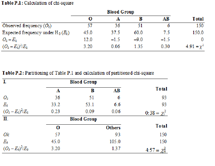
After a general conclusion is drawn regarding the presence of association in a contingency table by using the usual chi-square test, partitioning is used to obtain a focused conclusion regarding which particular category (or a set of categories) is causing the association. It is also possible that the overall chi-square test indicates no association but partitioning reveals some association somewhere. We use data in Table P.1 for illustrating partitioning of chi-square that shows the observed number of AIDS subjects with different blood groups (O, A, B, AB) from a population where these groups are in the ratio 6:5:8:1. These ratios provide H0: p1 = 6/20 = 0.30, p2 = 5/20 = 0.25. p3 = 8/20 = 0.40 and p4 = 1/20 = 0.05. Expected frequencies are based on these probabilities. The objective is to find whether or not the blood group pattern in AIDS cases is the same as in the population.
In this example, df = K – 1 = 4 – 1 = 3. Calculations are also presented in Table P.1, which show χ2 = 4.91. A relevant statistical software package automatically compares the calculated value of χ2 with its known distribution for 3 df and gives P = 0.178. Thus, the value 4.91 of χ2 obtained for these data is not all that unlikely when H0 is true. That is, the frequencies observed in different blood groups in the example are not very inconsistent with H0. The sample values do not provide sufficient evidence against H0 and so cannot be rejected. A preponderance of any blood group in cases of AIDS cannot be concluded on the basis of this sample when this method is used.
Examination of the data in this example reveals that the observed frequency in blood group O is much higher than expected from the pattern in the general population (57 vs 45) and the other differences are not as large. To check that this really is so, check whether the pattern in blood groups A, B, and AB (combined) is nearly the same as expected, and then check the difference in blood group O. The corresponding null hypotheses are
H01: A, B, and AB are in the ratio 5:8:1, and
H02: p1 = 6/20 = 0.3 for blood group O, p2 + p3 + p4 = 14/20 = 0.7 for the other three groups combined.
The former ratio is the same as in our example and the latter ratio combines A, B, and AB. Not stating H01 in terms of π is deliberate because that might give rise to confusion. The sum of πs in all contingency tables should be 1 and therefore the same πs cannot be used for the three cells covered by H01.
For these two null hypotheses, calculations for χ2 are shown in Table P.2. The division of the earlier four-cell table into two tables as shown is called partitioning. The first partition gives= 0.38 with 3 – 1 = 2 df, and from a software package P = 0.83 for this value of χ2. Since it is more than 0.05, H01 cannot be rejected at 5% level of significance, i.e., the evidence is not sufficient to conclude that the pattern of blood groups A, B, and AB in AIDS cases is not the same as in the general population. ... ...
For final and full version, see
Concise Encyclopedia of Biostatistics for Medical Professionals
Concise Encyclopedia of Biostatistics for Medical Professionals)
Partitioning of chi-square and of table, see also chi-square – overall
After a general conclusion is drawn regarding the presence of association in a contingency table by using the usual chi-square test, partitioning is used to obtain a focused conclusion regarding which particular category (or a set of categories) is causing the association. It is also possible that the overall chi-square test indicates no association but partitioning reveals some association somewhere. We use data in Table P.1 for illustrating partitioning of chi-square that shows the observed number of AIDS subjects with different blood groups (O, A, B, AB) from a population where these groups are in the ratio 6:5:8:1. These ratios provide H0: p1 = 6/20 = 0.30, p2 = 5/20 = 0.25. p3 = 8/20 = 0.40 and p4 = 1/20 = 0.05. Expected frequencies are based on these probabilities. The objective is to find whether or not the blood group pattern in AIDS cases is the same as in the population.
In this example, df = K – 1 = 4 – 1 = 3. Calculations are also presented in Table P.1, which show χ2 = 4.91. A relevant statistical software package automatically compares the calculated value of χ2 with its known distribution for 3 df and gives P = 0.178. Thus, the value 4.91 of χ2 obtained for these data is not all that unlikely when H0 is true. That is, the frequencies observed in different blood groups in the example are not very inconsistent with H0. The sample values do not provide sufficient evidence against H0 and so cannot be rejected. A preponderance of any blood group in cases of AIDS cannot be concluded on the basis of this sample when this method is used.
Examination of the data in this example reveals that the observed frequency in blood group O is much higher than expected from the pattern in the general population (57 vs 45) and the other differences are not as large. To check that this really is so, check whether the pattern in blood groups A, B, and AB (combined) is nearly the same as expected, and then check the difference in blood group O. The corresponding null hypotheses are
H01: A, B, and AB are in the ratio 5:8:1, and
H02: p1 = 6/20 = 0.3 for blood group O, p2 + p3 + p4 = 14/20 = 0.7 for the other three groups combined.
The former ratio is the same as in our example and the latter ratio combines A, B, and AB. Not stating H01 in terms of π is deliberate because that might give rise to confusion. The sum of πs in all contingency tables should be 1 and therefore the same πs cannot be used for the three cells covered by H01.
For these two null hypotheses, calculations for χ2 are shown in Table P.2. The division of the earlier four-cell table into two tables as shown is called partitioning. The first partition gives= 0.38 with 3 – 1 = 2 df, and from a software package P = 0.83 for this value of χ2. Since it is more than 0.05, H01 cannot be rejected at 5% level of significance, i.e., the evidence is not sufficient to conclude that the pattern of blood groups A, B, and AB in AIDS cases is not the same as in the general population. ... ...
For final and full version, see
Concise Encyclopedia of Biostatistics for Medical Professionals
