(This is a draft and truncated version - for final and full version, see
Concise Encyclopedia of Biostatistics for Medical Professionals)
time series, see also periodogram, autoregressive moving average (ARMA) models
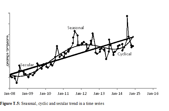
Recording the values of a variable at regular intervals over a long period of time gives rise to what is known as a time series. The observed movement and fluctuations within such a time series are generally made up of four components: (i) “secular trend” (the underlying smooth movement of a time series); (ii) seasonal variation; (iii) cyclical variation; and (iv) irregular variation called random. For example, the incidence of an infectious disease recorded monthly over several years in a population is a time series, where all these components may operate. In some time series, such as on incidence of some noncommunicable diseases, one or more of these components may be absent.
The primary purpose of studying time series is to explore and understand the trend over time, and sometimes to forecast values for the near future. Time series analysis comprises decomposing the series into seasonal, cyclical and secular trend – the remaining being random variation as just mentioned. Secular trend provides the long-term trend such as declining incidence of infectious diseases over the past 50 years. This trend is generally assumed linear that implies a constant rate of either growth in case of increase or of decay in case of decrease. The systematic variation could be cyclic such as we have 5-year cycle for dengue in India similar to the one depicted in Figure T.5. Parainfluenza is seen to have 2-year cycle [1] and dengue hemorrhagic fever a 5-year cycle in Latin America [2]. Seasonal trend is mostly within a year such as of swine flu occurring at the start of winter and of dengue with peak around the month of October in India each year as is clear from the Figure T.5. Such cyclic trend is visibly seen each day as circadian rhythm in blood pressure, heart rate, etc., or when a drug is taken such as three times a day. It is necessary that the hourly/ daily/weekly/ monthly values are available to study these components, and any time series has to be necessarily long for any adequate analysis, that is for say at least values for 50 time points.
Time series models are very useful for short range forecasting problems. They assume that whatever forces have influenced the variables in question in the recent past will continue to operate in the near future. Because of the complexity due to seasonal, cyclical and secular trend, forecasting in time series setup has to follow certain steps. As a first step, the series is smoothened so that the random variation is removed as much as possible. This involves some form of local averaging such as moving average that tends to cancel out the negative and positive irregular (random) component. If real outliers are present, perhaps the local median of few successive values can be tried in place of the arithmetic mean generally used in moving ‘average’. The appropriate lag for this is identified by periodogram analysis. Other smoothing methods such as cubic splines can also be used. Being local, these methods tend to highlight seasonal pattern but not cyclical pattern. The cyclical pattern is explored mostly with trigonometric functions such as sine waves. For secular trend, regular regression methods can be tried – simple linear if the trend is anticipated to follow linear trend, or curvilinear if the long-term trend seems like following a curve.
In analyzing time series data, it is necessary ... ...
For final and full version, see
Concise Encyclopedia of Biostatistics for Medical Professionals
Concise Encyclopedia of Biostatistics for Medical Professionals)
time series, see also periodogram, autoregressive moving average (ARMA) models
Recording the values of a variable at regular intervals over a long period of time gives rise to what is known as a time series. The observed movement and fluctuations within such a time series are generally made up of four components: (i) “secular trend” (the underlying smooth movement of a time series); (ii) seasonal variation; (iii) cyclical variation; and (iv) irregular variation called random. For example, the incidence of an infectious disease recorded monthly over several years in a population is a time series, where all these components may operate. In some time series, such as on incidence of some noncommunicable diseases, one or more of these components may be absent.
The primary purpose of studying time series is to explore and understand the trend over time, and sometimes to forecast values for the near future. Time series analysis comprises decomposing the series into seasonal, cyclical and secular trend – the remaining being random variation as just mentioned. Secular trend provides the long-term trend such as declining incidence of infectious diseases over the past 50 years. This trend is generally assumed linear that implies a constant rate of either growth in case of increase or of decay in case of decrease. The systematic variation could be cyclic such as we have 5-year cycle for dengue in India similar to the one depicted in Figure T.5. Parainfluenza is seen to have 2-year cycle [1] and dengue hemorrhagic fever a 5-year cycle in Latin America [2]. Seasonal trend is mostly within a year such as of swine flu occurring at the start of winter and of dengue with peak around the month of October in India each year as is clear from the Figure T.5. Such cyclic trend is visibly seen each day as circadian rhythm in blood pressure, heart rate, etc., or when a drug is taken such as three times a day. It is necessary that the hourly/ daily/weekly/ monthly values are available to study these components, and any time series has to be necessarily long for any adequate analysis, that is for say at least values for 50 time points.
Time series models are very useful for short range forecasting problems. They assume that whatever forces have influenced the variables in question in the recent past will continue to operate in the near future. Because of the complexity due to seasonal, cyclical and secular trend, forecasting in time series setup has to follow certain steps. As a first step, the series is smoothened so that the random variation is removed as much as possible. This involves some form of local averaging such as moving average that tends to cancel out the negative and positive irregular (random) component. If real outliers are present, perhaps the local median of few successive values can be tried in place of the arithmetic mean generally used in moving ‘average’. The appropriate lag for this is identified by periodogram analysis. Other smoothing methods such as cubic splines can also be used. Being local, these methods tend to highlight seasonal pattern but not cyclical pattern. The cyclical pattern is explored mostly with trigonometric functions such as sine waves. For secular trend, regular regression methods can be tried – simple linear if the trend is anticipated to follow linear trend, or curvilinear if the long-term trend seems like following a curve.
In analyzing time series data, it is necessary ... ...
For final and full version, see
Concise Encyclopedia of Biostatistics for Medical Professionals
